Climate change is impacting the way people live around the world
::: {.cell .markdown}
Higher highs, lower lows, storms, and smoke – we’re all feeling the
effects of climate change. In this workflow, you will take a look at
trends in temperature over time in Rapid City, SD.
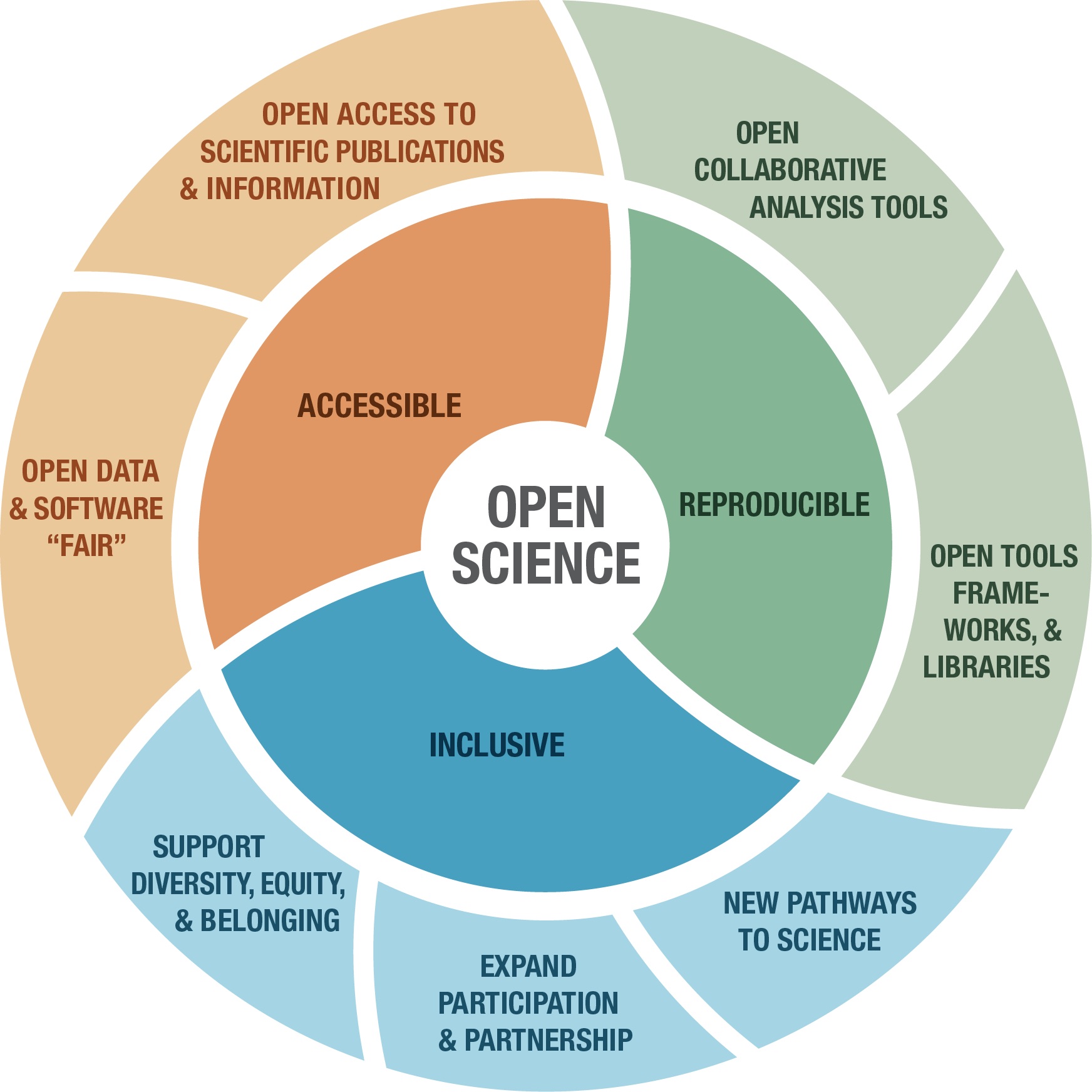
Open reproducible
science
makes scientific methods, data and outcomes available to everyone. That
means that everyone who wants should be able to find, read,
understand, and run your workflows for themselves.
Few if any science projects are 100% open and reproducible (yet!).
However, members of the open science community have developed open
source tools and practices that can help you move toward that goal. You
will learn about many of those tools in the Intro to Earth Data Science
textbook.
Don’t worry about learning all the tools at once – we’ve picked a few
for you to get started with.
Create a
new Markdown cell below this one using the + Markdown button in the
upper left.
In the
new cell, answer the following questions using a numbered list in
Markdown:
In 1-2 sentences, define open reproducible science.
In 1-2 sentences, choose one of the open source tools that you
have learned about (i.e. Shell, Git/GitHub, Jupyter Notebook,
Python) and explain how it supports open reproducible science.
Open reproducible science is about making research, it's methods and outcomes, available to anyone. This includes that the research can be repeated, the data used is available to the public, and there is transparency around the methods and results.
GitHub supports open and reproducible science because it allows a space where findings can be shared easily with the public and other researchers. With GitHub's functionality of codespaces and the ability to fork code, it allows for others to take your code, use it, add onto it, and continue to progress research.
Create a
new Markdown cell below this one using the ESC + b
keyboard shortcut.
In the new
cell, answer the following question in a Markdown quote: In 1-2
sentences, does this Jupyter Notebook file have a machine-readable name?
Explain your answer.
This Jupyter notebook doesn't have a machine-readable name because it has spaces and an exclimation point in the name.
Below is a scientific Python workflow. But something’s wrong – The code
won’t run! Your task is to follow the instructions below to clean and
debug the Python code below so that it runs.
Tip
Don’t worry if you can’t solve every bug right away. We’ll get there!
The most important thing is to identify problems with the code and
write high-quality GitHub
Issues.
At the end, you’ll repeat the workflow for a location and
measurement of your choosing.
Alright! Let’s clean up this code. First things first…
Python packages let you use code written by experts around the world
Because Python is open source, lots of different people and
organizations can contribute (including you!). Many contributions are in
the form of packages which do not come with a standard Python
download.
Correct the typo below to properly import the pandas package under
its alias pd.
Run the cell to import pandas
NOTE: **Run your code in the right **environment** to avoid import
errors**
We’ve created a coding environment for you to use that already has
all the software and libraries you will need! When you try to run some
code, you may be prompted to select a kernel. The kernel
refers to the version of Python you are using. You should use the
base kernel, which should be the default option.
In [1]:
# Import pandasimportpandasaspd
Once you have run the cell above and imported pandas, run the cell
below. It is a test cell that will tell you if you completed the task
successfully. If a test cell isn’t working the way you expect, check
that you ran your code immediately before running the test.
In [2]:
# DO NOT MODIFY THIS TEST CELLpoints=0try:pd.DataFrame()points+=5print('\u2705 Great work! You correctly imported the pandas library.')except:print('\u274C Oops - pandas was not imported correctly.')print('You earned {} of 5 points for importing pandas'.format(points))
✅ Great work! You correctly imported the pandas library.
You earned 5 of 5 points for importing pandas
There are more Earth Observation data online than any one person could ever look at
Here we’re using the NOAA National Centers for Environmental Information
(NCEI) Access Data
Service
application progamming interface (API) to request data from their web
servers. We will be using data collected as part of the Global
Historical Climatology Network daily (GHCNd) from their Climate Data
Online library program at
NOAA.
In the cell below, write a 2-3 sentence description of the data
source. You should describe:
who takes the data
where the data were taken
what the maximum temperature units are
how the data are collected
Include a citation of the data (HINT: See the ‘Data Citation’
tab on the GHCNd overview page).
The data is taken from 30 different sources at climate stations around the world. Over 25,000 stations are regularly updated with observations from within roughly the last month. The dataset includes observations from World Meteorological Organization, Cooperative, and CoCoRaHS networks. NOAA's National Centers for Environmental Information houses this data. The maximum temperature units is tenths of degrees C. The dataset is also routinely reconstructed (usually every week) from its roughly 30 data sources to ensure that GHCN-Daily is generally in sync with its growing list of constituent sources. The data is collected from climate stations around the world.
Citation:
Menne, Matthew J., Imke Durre, Bryant Korzeniewski, Shelley McNeill, Kristy Thomas, Xungang Yin, Steven Anthony, Ron Ray, Russell S. Vose, Byron E.Gleason, and Tamara G. Houston (2012): Global Historical Climatology Network - Daily (GHCN-Daily), Version 3. [indicate subset used]. NOAA National Climatic Data Center. doi:10.7289/V5D21VHZ [May 13, 2024].
You can access NCEI GHCNd Data from the internet using its API 🖥️ 📡 🖥️
The cell below contains the URL for the data you will use in this part
of the notebook. We created this URL by generating what is called an
API endpoint using the NCEI API
documentation.
Note
An application programming interface (API) is a way for two or
more computer programs or components to communicate with each other.
It is a type of software interface, offering a service to other pieces
of software (Wikipedia).
However, we still have a problem - we can’t get the URL back later on
because it isn’t saved in a variable. In other words, we need to
give the url a name so that we can request in from Python later (sadly,
Python has no ‘hey what was that thingy I typed yesterday?’ function).
Pick an expressive variable name for the URL. HINT: click on the
Variables button up top to see all your variables. Your new url
variable will not be there until you define it and run the code
Reformat the URL so that it adheres to the 79-character PEP-8
line
limit.You
should see two vertical lines in each cell - don’t let your code
go past the second line
At the end of the cell where you define your url variable, call
your variable (type out its name) so it can be tested.
In [3]:
# Getting data from NCEI for Rapid City, COrapidcityurl=('https://www.ncei.noaa.gov/access/services/data/v1?''dataset=daily-summaries''&dataTypes=TOBS,PRCP''&stations=USC00396947''&startDate=1949-10-01''&endDate=2024-05-03''&includeStationName=true''&includeStationLocation=1''&units=standard')rapidcityurl
# DO NOT MODIFY THIS TEST CELLresp_url=_points=0iftype(resp_url)==str:points+=3print('\u2705 Great work! You correctly called your url variable.')else:print('\u274C Oops - your url variable was not called correctly.')iflen(resp_url)==218:points+=3print('\u2705 Great work! Your url is the correct length.')else:print('\u274C Oops - your url variable is not the correct length.')print('You earned {} of 6 points for defining a url variable'.format(points))
✅ Great work! You correctly called your url variable.
✅ Great work! Your url is the correct length.
You earned 6 of 6 points for defining a url variable
The pandas library you imported can download data from the internet
directly into a type of Python object called a DataFrame. In the
code cell below, you can see an attempt to do just this. But there are
some problems…
You’re ready to fix some code!
Your task is to:
Leave a space between the # and text in the comment and try
making the comment more informative
Make any changes needed to get this code to run. HINT: The
my_url variable doesn’t exist - you need to replace it with the
variable name you chose.
Modify the .read_csv() statement to include the following
parameters:
index_col='DATE' – this sets the DATE column as the index.
Needed for subsetting and resampling later on
parse_dates=True – this lets python know that you are
working with time-series data, and values in the indexed
column are date time objects
na_values=['NaN'] – this lets python know how to handle
missing values
Clean up the code by using expressive variable names,
expressive column names, PEP-8 compliant code, and
descriptive comments
Make sure to call your DataFrame by typing it’s name as the last
line of your code cell Then, you will be able to run the test cell
below and find out if your answer is correct.
In [5]:
# creating a data frame for Rapid Cityrapidcity_df=pd.read_csv(rapidcityurl,index_col='DATE',parse_dates=True,na_values=['NaN'])rapidcity_df
Out[5]:
STATION
NAME
LATITUDE
LONGITUDE
ELEVATION
PRCP
TOBS
DATE
1949-10-01
USC00396947
RAPID CITY 4 NW, SD US
44.12055
-103.28417
1060.4
0.00
51.0
1949-10-02
USC00396947
RAPID CITY 4 NW, SD US
44.12055
-103.28417
1060.4
0.00
51.0
1949-10-03
USC00396947
RAPID CITY 4 NW, SD US
44.12055
-103.28417
1060.4
0.00
52.0
1949-10-04
USC00396947
RAPID CITY 4 NW, SD US
44.12055
-103.28417
1060.4
0.00
45.0
1949-10-05
USC00396947
RAPID CITY 4 NW, SD US
44.12055
-103.28417
1060.4
0.00
50.0
...
...
...
...
...
...
...
...
2024-04-28
USC00396947
RAPID CITY 4 NW, SD US
44.12055
-103.28417
1060.4
0.00
NaN
2024-04-29
USC00396947
RAPID CITY 4 NW, SD US
44.12055
-103.28417
1060.4
0.37
30.0
2024-04-30
USC00396947
RAPID CITY 4 NW, SD US
44.12055
-103.28417
1060.4
0.00
44.0
2024-05-01
USC00396947
RAPID CITY 4 NW, SD US
44.12055
-103.28417
1060.4
0.00
33.0
2024-05-02
USC00396947
RAPID CITY 4 NW, SD US
44.12055
-103.28417
1060.4
0.35
39.0
26109 rows × 7 columns
In [6]:
# DO NOT MODIFY THIS TEST CELLtmax_df_resp=_points=0ifisinstance(tmax_df_resp,pd.DataFrame):points+=1print('\u2705 Great work! You called a DataFrame.')else:print('\u274C Oops - make sure to call your DataFrame for testing.')print('You earned {} of 2 points for downloading data'.format(points))
✅ Great work! You called a DataFrame.
You earned 1 of 2 points for downloading data
HINT: Check out the type() function below - you can use it to check
that your data is now in DataFrame type object
In [7]:
# Check that the data was imported into a pandas DataFrametype(rapidcity_df)
Out[7]:
pandas.core.frame.DataFrame
Clean up your DataFrame
Use double brackets to only select the columns you want in your
DataFrame
Make sure to call your DataFrame by typing it’s name as the last
line of your code cell Then, you will be able to run the test cell
below and find out if your answer is correct.
In [8]:
# Checking column names to know all columns in datarapidcity_df.columns
# Rewriting data frame to only have precipitations and TOBS datarapidcity_df=rapidcity_df[['PRCP','TOBS']]rapidcity_df
Out[9]:
PRCP
TOBS
DATE
1949-10-01
0.00
51.0
1949-10-02
0.00
51.0
1949-10-03
0.00
52.0
1949-10-04
0.00
45.0
1949-10-05
0.00
50.0
...
...
...
2024-04-28
0.00
NaN
2024-04-29
0.37
30.0
2024-04-30
0.00
44.0
2024-05-01
0.00
33.0
2024-05-02
0.35
39.0
26109 rows × 2 columns
In [10]:
# DO NOT MODIFY THIS TEST CELLtmax_df_resp=_points=0summary=[round(val,2)forvalintmax_df_resp.mean().values]ifsummary==[0.05,54.53]:points+=4print('\u2705 Great work! You correctly downloaded data.')else:print('\u274C Oops - your data are not correct.')print('You earned {} of 5 points for downloading data'.format(points))
❌ Oops - your data are not correct.
You earned 0 of 5 points for downloading data
Plot the precpitation column (PRCP) vs time to explore the data
Plotting in Python is easy, but not quite this easy:
In [11]:
# Plotting Rapid City PRCP and TOBS
rapidcity_df.plot()
Out[11]:
<Axes: xlabel='DATE'>
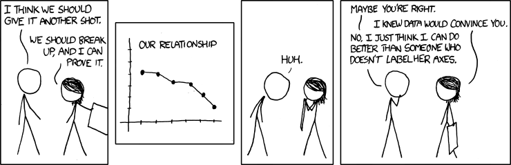
****Label and describe your plots****
Source: https://xkcd.com/833
Make sure each plot has:
A title that explains where and when the data are from
x- and y- axis labels with units where appropriate
A legend where appropriate
You’ll always need to add some instructions on labels and how you want
your plot to look.
Your task:
Change dataframe to yourDataFrame name.
Change y= to the name of your observed temperature column
name.
Use the title, ylabel, and xlabel parameters to add key text
to your plot.
Adjust the size of your figure using figsize=(x,y) where x is
figure width and y is figure height
HINT: labels have to be a type in Python called a string.
You can make a string by putting quotes around your label, just like
the column names in the sample code (eg y='TOBS').
In [12]:
# Plotting Daily Observed Temperature for Rapid City from 1944-2024rapidcity_df.plot(y='TOBS',title='Rapid City Daily Observed Temperature 1944-2024',xlabel='Date',ylabel='Temperature (F)',legend=False,color='blue',figsize=(10,5),fontsize=14)
Out[12]:
<Axes: title={'center': 'Rapid City Daily Observed Temperature 1944-2024'}, xlabel='Date', ylabel='Temperature (F)'>
Want an EXTRA CHALLENGE?
There are many other things you can do to customize your plot. Take a
look at the pandas plotting
galleries
and the documentation of
plot
to see if there’s other changes you want to make to your plot. Some
possibilities include:
Remove the legend since there’s only one data series
Increase the figure size
Increase the font size
Change the colors
Use a bar graph instead (usually we use lines for time series, but
since this is annual it could go either way)
Add a trend line
Not sure how to do any of these? Try searching the internet, or asking
an AI!
Convert units
Modify the code below to add a column that includes temperature in
Celsius. The code below was written by your colleague. Can you fix
this so that it correctly calculates temperature in Celsius and adds a
new column?
In [13]:
# Convert to celciusrapidcity_df.loc[:,'TCel']=(rapidcity_df['TOBS']-32)*5/9rapidcity_df
/tmp/ipykernel_6497/1789627478.py:2: SettingWithCopyWarning:
A value is trying to be set on a copy of a slice from a DataFrame.
Try using .loc[row_indexer,col_indexer] = value instead

See the caveats in the documentation: https://pandas.pydata.org/pandas-docs/stable/user_guide/indexing.html#returning-a-view-versus-a-copy
  rapidcity_df.loc[:,'TCel'] = (rapidcity_df['TOBS'] - 32) * 5 / 9
Out[13]:
PRCP
TOBS
TCel
DATE
1949-10-01
0.00
51.0
10.555556
1949-10-02
0.00
51.0
10.555556
1949-10-03
0.00
52.0
11.111111
1949-10-04
0.00
45.0
7.222222
1949-10-05
0.00
50.0
10.000000
...
...
...
...
2024-04-28
0.00
NaN
NaN
2024-04-29
0.37
30.0
-1.111111
2024-04-30
0.00
44.0
6.666667
2024-05-01
0.00
33.0
0.555556
2024-05-02
0.35
39.0
3.888889
26109 rows × 3 columns
In [14]:
# DO NOT MODIFY THIS TEST CELLtmax_df_resp=_points=0ifisinstance(tmax_df_resp,pd.DataFrame):points+=1print('\u2705 Great work! You called a DataFrame.')else:print('\u274C Oops - make sure to call your DataFrame for testing.')summary=[round(val,2)forvalintmax_df_resp.mean().values]ifsummary==[0.05,54.53,12.52]:points+=4print('\u2705 Great work! You correctly converted to Celcius.')else:print('\u274C Oops - your data are not correct.')print('You earned {} of 5 points for converting to Celcius'.format(points))
✅ Great work! You called a DataFrame.
❌ Oops - your data are not correct.
You earned 1 of 5 points for converting to Celcius
Want an EXTRA CHALLENGE?
As you did above, rewrite the code to be more expressive
Using the code below as a framework, write and apply a
function that converts to Celcius. > Functions let you
reuse code you have already written
You should also rewrite this function and parameter names to be
more expressive.
In [15]:
# Creating a function to convert from fahrenheit to celsiusdefto_celsius(fahrenheit):"""Convert temperature to Celsius"""return(fahrenheit-32)*5/9# Displaying dataframe with new column, celsiusrapidcity_df['celsius']=rapidcity_df['TOBS'].apply(to_celsius)rapidcity_df
/tmp/ipykernel_6497/2859914288.py:7: SettingWithCopyWarning:
A value is trying to be set on a copy of a slice from a DataFrame.
Try using .loc[row_indexer,col_indexer] = value instead

See the caveats in the documentation: https://pandas.pydata.org/pandas-docs/stable/user_guide/indexing.html#returning-a-view-versus-a-copy
  rapidcity_df['celsius'] = rapidcity_df['TOBS'].apply(to_celsius)
Often when working with time-series data you may want to focus on a
shorter window of time, or look at weekly, monthly, or annual summaries
to help make the analysis more manageable.
Read more
Read more about
subsetting
and
resampling
time-series data in our Learning Portal.
For this demonstration, we will look at the last 40 years worth of data
and resample to explore a summary from each year that data were
recorded.
Your task
Replace start-year and end-year with 1983 and 2023
Replace dataframe with the name of your data
Replace new_dataframe with something more expressive
Call your new variable
Run the cell
In [16]:
# Subset the datarapidcitysubset=rapidcity_df.loc['1983':'2023']rapidcitysubset
Out[16]:
PRCP
TOBS
TCel
celsius
DATE
1983-01-01
0.00
30.0
-1.111111
-1.111111
1983-01-02
0.00
29.0
-1.666667
-1.666667
1983-01-03
0.00
40.0
4.444444
4.444444
1983-01-04
0.00
33.0
0.555556
0.555556
1983-01-05
0.00
43.0
6.111111
6.111111
...
...
...
...
...
2023-12-27
0.31
32.0
0.000000
0.000000
2023-12-28
0.00
17.0
-8.333333
-8.333333
2023-12-29
0.00
28.0
-2.222222
-2.222222
2023-12-30
0.00
NaN
NaN
NaN
2023-12-31
0.00
NaN
NaN
NaN
13939 rows × 4 columns
In [17]:
# DO NOT MODIFY THIS TEST CELLdf_resp=_points=0ifisinstance(df_resp,pd.DataFrame):points+=1print('\u2705 Great work! You called a DataFrame.')else:print('\u274C Oops - make sure to call your DataFrame for testing.')summary=[round(val,2)forvalindf_resp.mean().values]ifsummary==[0.06,55.67,13.15]:points+=5print('\u2705 Great work! You correctly converted to Celcius.')else:print('\u274C Oops - your data are not correct.')print('You earned {} of 5 points for subsetting'.format(points))
✅ Great work! You called a DataFrame.
❌ Oops - your data are not correct.
You earned 1 of 5 points for subsetting
Here you will resample the 1983-2023 data to look the annual mean
values.
Resample your data
Replace new_dataframe with the variable you created in the cell
above where you subset the data
Replace 'TIME' with a 'W', 'M', or 'Y' depending on
whether you’re doing a weekly, monthly, or yearly summary
Replace STAT with a sum, min, max, or mean depending on
what kind of statistic you’re interested in calculating.
Replace resampled_data with a more expressive variable name
Call your new variable
Run the cell
In [18]:
# Resample the data to look at yearly mean valuesrapidyearly=rapidcitysubset.resample('YE').mean()rapidyearly
Out[18]:
PRCP
TOBS
TCel
celsius
DATE
1983-12-31
0.038849
59.302632
15.168129
15.168129
1984-12-31
0.026145
54.458182
12.476768
12.476768
1985-12-31
0.039091
50.691667
10.384259
10.384259
1986-12-31
0.069551
53.672673
12.040374
12.040374
1987-12-31
0.039011
56.988950
13.882750
13.882750
1988-12-31
0.028017
56.983240
13.879578
13.879578
1989-12-31
0.056359
38.072829
3.373794
3.373794
1990-12-31
0.039068
40.363112
4.646174
4.646174
1991-12-31
0.056875
39.945869
4.414372
4.414372
1992-12-31
0.036714
39.525862
4.181034
4.181034
1993-12-31
0.055881
35.522581
1.956989
1.956989
1994-12-31
0.034540
39.479769
4.155427
4.155427
1995-12-31
0.063609
39.150568
3.972538
3.972538
1996-12-31
0.058785
36.547486
2.526381
2.526381
1997-12-31
0.057634
38.825073
3.791707
3.791707
1998-12-31
0.068343
40.563739
4.757633
4.757633
1999-12-31
0.073104
41.688202
5.382335
5.382335
2000-12-31
0.050771
39.750751
4.305973
4.305973
2001-12-31
0.049639
43.371134
6.317297
6.317297
2002-12-31
0.036126
33.482143
0.823413
0.823413
2003-12-31
0.039186
40.455253
4.697363
4.697363
2004-12-31
0.030242
38.877828
3.821016
3.821016
2005-12-31
0.044620
40.627119
4.792844
4.792844
2006-12-31
0.042870
40.873278
4.929599
4.929599
2007-12-31
0.038515
34.806931
1.559406
1.559406
2008-12-31
0.025892
34.204969
1.224983
1.224983
2009-12-31
0.053828
35.871324
2.150735
2.150735
2010-12-31
0.056767
39.012384
3.895769
3.895769
2011-12-31
0.060282
40.313846
4.618803
4.618803
2012-12-31
0.019341
42.008746
5.560415
5.560415
2013-12-31
0.060685
38.392638
3.551466
3.551466
2014-12-31
0.057726
39.211310
4.006283
4.006283
2015-12-31
0.057260
41.351275
5.195153
5.195153
2016-12-31
0.039508
42.161644
5.645358
5.645358
2017-12-31
0.034082
41.013889
5.007716
5.007716
2018-12-31
0.057335
36.670732
2.594851
2.594851
2019-12-31
0.085056
36.159544
2.310858
2.310858
2020-12-31
0.044006
41.023438
5.013021
5.013021
2021-12-31
0.032225
40.363248
4.646249
4.646249
2022-12-31
0.028421
39.331395
4.072997
4.072997
2023-12-31
0.046313
40.144578
4.524766
4.524766
In [19]:
# DO NOT MODIFY THIS TEST CELLdf_resp=_points=0ifisinstance(df_resp,pd.DataFrame):points+=1print('\u2705 Great work! You called a DataFrame.')else:print('\u274C Oops - make sure to call your DataFrame for testing.')summary=[round(val,2)forvalindf_resp.mean().values]ifsummary==[0.06,55.37,12.99]:points+=5print('\u2705 Great work! You correctly converted to Celcius.')else:print('\u274C Oops - your data are not correct.')print('You earned {} of 5 points for resampling'.format(points))
✅ Great work! You called a DataFrame.
❌ Oops - your data are not correct.
You earned 1 of 5 points for resampling
Plot your resampled data
In [20]:
# Plot mean annual temperature values from 1983 to 2023rapidyearly.plot(y='TOBS',title='Rapid City Annual Mean Temperatures 1983-2023',xlabel='Year',ylabel='Temperature (F)',legend=False,color='blue',figsize=(10,5),fontsize=14)
Out[20]:
<Axes: title={'center': 'Rapid City Annual Mean Temperatures 1983-2023'}, xlabel='Year', ylabel='Temperature (F)'>
Describe your plot
We like to use an approach called “Assertion-Evidence” for presenting
scientific results. There’s a lot of video tutorials and example talks
available on the Assertion-Evidence web
page. The main thing you need to
do now is to practice writing a message or headline rather
than descriptions or topic sentences for the plot you just made (what
they refer to as “visual evidence”).
For example, it would be tempting to write something like “A plot of
maximum annual temperature in Rapid City, Colorado over time
(1983-2023)”. However, this doesn’t give the reader anything to look
at, or explain why we made this particular plot (we know, you made
this one because we told you to)
Some alternatives for different plots of Rapid City temperature that
are more of a starting point for a presentation or conversation are:
Rapid City, SD experienced cooler than average temperatures in
1995
Temperatures in Rapid City, SD appear to be on the rise over the
past 40 years
Maximum annual temperatures in Rapid City, CO are becoming more
variable over the previous 40 years
We could back up some of these claims with further analysis included
later on, but we want to make sure that our audience has some guidance
on what to look for in the plot.
**Rapid City, CO colder than 40 years ago and temperatures continue to shift! ** 📰 🗞️ 📻
In the late eighties, Rapid City, Colorado experienced a drastic decrease in average annual temperature of almost 20 degrees fahrenheit. Today the annual mean remains low and is having more stark changes year to year.
Your turn: pick a new location and/or measurement to plot 🌏 📈
Below (or in a new notebook!), recreate the workflow you just did in a
place that interests you OR with a different measurement. See the
instructions above to adapt the URL that we created for Rapid City, CO
using the NCEI API. You will need to make your own new Markdown and Code
cells below this one, or create a new notebook.
Congratulations, you’re almost done with this coding challenge 🤩 – now make sure that your code is reproducible
If you didn’t already, go back to the code you modified about and
write more descriptive comments so the next person to use this
code knows what it does.
Make sure to Restart and Run all up at the top of your
notebook. This will clear all your variables and make sure that
your code runs in the correct order. It will also export your work
in Markdown format, which you can put on your website.
Always run your code start to finish before submitting!
Before you commit your work, make sure it runs reproducibly by
clicking:
Restart (this button won’t appear until you’ve run some code),
then
Below is some code that you can run that will save a Markdown file of
your work that is easily shareable and can be uploaded to GitHub Pages.
You can use it as a starting point for writing your portfolio post!
In [21]:
#Recreating with Rainier Paradise Ranger Station in Mount Rainier#USC00456898 46.7858 -121.7425 1654.1 WA RAINIER PARADISE RS rainierurl=('https://www.ncei.noaa.gov/access/services/data/v1?''dataset=daily-summaries''&dataTypes=TOBS,PRCP''&stations=USC00456898''&startDate=1916-12-01''&endDate=2024-05-12''&includeStationName=true''&includeStationLocation=1''&units=standard')rainierurl
# creating a data frame for Rainierrainier_df=pd.read_csv(rainierurl,index_col='DATE',parse_dates=True,na_values=['NaN'])rainier_df
Out[22]:
STATION
NAME
LATITUDE
LONGITUDE
ELEVATION
PRCP
TOBS
DATE
1916-12-01
USC00456898
RAINIER PARADISE RANGER STATION, WA US
46.78639
-121.74222
1650.5
NaN
29.0
1916-12-02
USC00456898
RAINIER PARADISE RANGER STATION, WA US
46.78639
-121.74222
1650.5
NaN
28.0
1916-12-03
USC00456898
RAINIER PARADISE RANGER STATION, WA US
46.78639
-121.74222
1650.5
NaN
21.0
1916-12-04
USC00456898
RAINIER PARADISE RANGER STATION, WA US
46.78639
-121.74222
1650.5
NaN
23.0
1916-12-05
USC00456898
RAINIER PARADISE RANGER STATION, WA US
46.78639
-121.74222
1650.5
NaN
22.0
...
...
...
...
...
...
...
...
2024-05-08
USC00456898
RAINIER PARADISE RANGER STATION, WA US
46.78639
-121.74222
1650.5
NaN
NaN
2024-05-09
USC00456898
RAINIER PARADISE RANGER STATION, WA US
46.78639
-121.74222
1650.5
NaN
54.0
2024-05-10
USC00456898
RAINIER PARADISE RANGER STATION, WA US
46.78639
-121.74222
1650.5
0.0
61.0
2024-05-11
USC00456898
RAINIER PARADISE RANGER STATION, WA US
46.78639
-121.74222
1650.5
0.0
59.0
2024-05-12
USC00456898
RAINIER PARADISE RANGER STATION, WA US
46.78639
-121.74222
1650.5
0.0
54.0
35888 rows × 7 columns
In [23]:
# Keeping only precipitation and TOBS columnsrainier_df=rainier_df[['PRCP','TOBS']]rainier_df
Out[23]:
PRCP
TOBS
DATE
1916-12-01
NaN
29.0
1916-12-02
NaN
28.0
1916-12-03
NaN
21.0
1916-12-04
NaN
23.0
1916-12-05
NaN
22.0
...
...
...
2024-05-08
NaN
NaN
2024-05-09
NaN
54.0
2024-05-10
0.0
61.0
2024-05-11
0.0
59.0
2024-05-12
0.0
54.0
35888 rows × 2 columns
In [24]:
# Plotting Rainier Daily Observed Temperaturerainier_df.plot(y='TOBS',title='Rainier Paradise Ranger Station City Daily Observed Temperature 1916-2024',xlabel='Date',ylabel='Temperature (F)',legend=False,color='blue',figsize=(10,5),fontsize=14)
Out[24]:
<Axes: title={'center': 'Rainier Paradise Ranger Station City Daily Observed Temperature 1916-2024'}, xlabel='Date', ylabel='Temperature (F)'>
In [25]:
# Convert to celciusrainier_df.loc[:,'TCel']=(rainier_df['TOBS']-32)*5/9rainier_df
/tmp/ipykernel_6497/1784484435.py:2: SettingWithCopyWarning:
A value is trying to be set on a copy of a slice from a DataFrame.
Try using .loc[row_indexer,col_indexer] = value instead

See the caveats in the documentation: https://pandas.pydata.org/pandas-docs/stable/user_guide/indexing.html#returning-a-view-versus-a-copy
  rainier_df.loc[:,'TCel'] = (rainier_df['TOBS'] - 32) * 5 / 9
Out[25]:
PRCP
TOBS
TCel
DATE
1916-12-01
NaN
29.0
-1.666667
1916-12-02
NaN
28.0
-2.222222
1916-12-03
NaN
21.0
-6.111111
1916-12-04
NaN
23.0
-5.000000
1916-12-05
NaN
22.0
-5.555556
...
...
...
...
2024-05-08
NaN
NaN
NaN
2024-05-09
NaN
54.0
12.222222
2024-05-10
0.0
61.0
16.111111
2024-05-11
0.0
59.0
15.000000
2024-05-12
0.0
54.0
12.222222
35888 rows × 3 columns
In [26]:
# creating subset from 1980 to 2023rainiersubset=rainier_df.loc['1980':'2023']rainiersubset
Out[26]:
PRCP
TOBS
TCel
DATE
1980-01-01
1.29
29.0
-1.666667
1980-01-02
0.08
31.0
-0.555556
1980-01-03
0.74
18.0
-7.777778
1980-01-04
0.10
21.0
-6.111111
1980-01-05
1.58
18.0
-7.777778
...
...
...
...
2023-12-27
NaN
NaN
NaN
2023-12-28
NaN
36.0
2.222222
2023-12-29
0.00
40.0
4.444444
2023-12-30
0.20
34.0
1.111111
2023-12-31
0.39
32.0
0.000000
15280 rows × 3 columns
In [27]:
# Resampling to get only mean yearly values rainieryearly=rainiersubset.resample('YE').mean()rainieryearly
Out[27]:
PRCP
TOBS
TCel
DATE
1980-12-31
0.340847
34.983516
1.657509
1981-12-31
0.337315
36.912088
2.728938
1982-12-31
0.316418
34.668524
1.482513
1983-12-31
0.355205
35.173077
1.762821
1984-12-31
0.337637
33.704918
0.947177
1985-12-31
0.228000
35.640110
2.022283
1986-12-31
0.310932
38.142466
3.412481
1987-12-31
0.199331
39.781818
4.323232
1988-12-31
0.328297
37.186301
2.881279
1989-12-31
0.274848
35.632597
2.018109
1990-12-31
0.405439
35.107042
1.726135
1991-12-31
0.347582
36.430137
2.461187
1992-12-31
0.272932
37.699454
3.166363
1993-12-31
0.218822
33.498630
0.832572
1994-12-31
0.384620
35.877483
2.154157
1995-12-31
0.382644
35.853968
2.141093
1996-12-31
0.354772
36.933824
2.741013
1997-12-31
0.398710
35.944984
2.191658
1998-12-31
0.330840
36.889205
2.716225
1999-12-31
0.342132
35.739394
2.077441
2000-12-31
0.261652
33.385382
0.769657
2001-12-31
0.332028
33.288401
0.715778
2002-12-31
0.289858
37.241379
2.911877
2003-12-31
0.357840
35.927419
2.181900
2004-12-31
0.301335
40.064706
4.480392
2005-12-31
0.297229
38.962536
3.868076
2006-12-31
0.378636
38.075758
3.375421
2007-12-31
0.299623
37.391975
2.995542
2008-12-31
0.318908
35.789272
2.105151
2009-12-31
0.264627
36.655052
2.586140
2010-12-31
0.276537
38.596330
3.664628
2011-12-31
0.370717
34.744681
1.524823
2012-12-31
0.339748
36.509434
2.505241
2013-12-31
0.286890
38.206294
3.447941
2014-12-31
0.345017
38.678457
3.710254
2015-12-31
0.321603
41.861314
5.478508
2016-12-31
0.375076
38.674658
3.708143
2017-12-31
0.297438
40.143791
4.524328
2018-12-31
0.385768
38.235880
3.464378
2019-12-31
0.256429
38.764331
3.757962
2020-12-31
0.488738
37.295276
2.941820
2021-12-31
0.340103
40.833333
4.907407
2022-12-31
0.227745
41.918301
5.510167
2023-12-31
0.232778
43.404669
6.335927
In [28]:
# Plot mean annual temperature values for Rainier from 1980 to 2023rainieryearly.plot(y='TOBS',title='Rainier Paradise Ranger Station Annual Mean Temperatures 1980-2023',xlabel='Year',ylabel='Temperature (F)',legend=False,color='blue',figsize=(10,5),fontsize=14)
Out[28]:
<Axes: title={'center': 'Rainier Paradise Ranger Station Annual Mean Temperatures 1980-2023'}, xlabel='Year', ylabel='Temperature (F)'>
**Temperatures on the rise in Mount Rainier, WA over the last 40 years! ** 📰 🗞️ 📻
Over the last 40 years, Mount Rainier has experienced many drastic changes in temperature. Today we can see that both the extreme lows and extreme highs are increasing.